Part Four – Pretending to Be Super Smart
[The entire report can be downloaded as PDF, flood_years-r0-20241201.pdf]
[The start: https://www.scienceisjunk.com/the-100-year-flood-a-skeptical-inquiry-part-1/]
Probability theory is full of theorems that work “for very large n”, the number of samples in a sequence. Taken to the limit, the observed maximum from a large data set should fall in line to one of a few simple-ish distributions, no matter the original distribution. The theory is air-tight, at the limit. But it leaves a person living in a real particular location and time, with explicitly limited sets of data, asking, “How many ‘n’ is large enough? How small of an ‘n’ is too dangerous to use?”
The Fancy-Pants Way to 100 Year Floods
We will apply one analysis method to data from near Nashville, Tennessee. This is a relatively long and high-quality data set. (There are “only” 213 missing values in the raw precipitation data from 1948 onward.) To start, I insist we use data only through 2009, for a reason that will become clear.

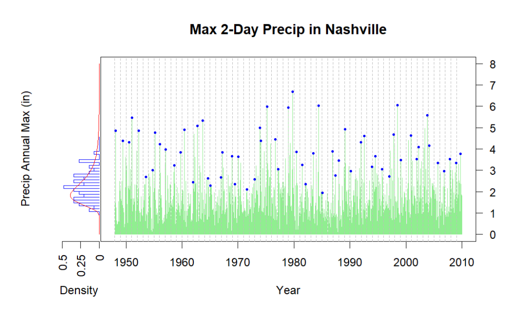
In the busy plot we have combined daily rain data for Nashville, select annual peaks marked by blue dots, and a histogram of all the annual maximums plotted up the left side[1]. A red curve is fitted to the histogram. This curve is from what is called the “generalized extreme value distribution”. It gives us probabilities of extreme values, higher than the maximums already observed, just like the exponential or power law plots of the first section. But the GEV has formal theoretical rigor behind it: for enough samples, the solution is exact, if certain requirements are met and we have all eternity to sit and watch.
Since we don’t have eternity to wait or an infinite amount of data from the past, we need some idea how the size of our actual data set affects our answer. It’s a straightforward thing to calculate “confidence” intervals based on the assumed distribution and how many samples we got from it.

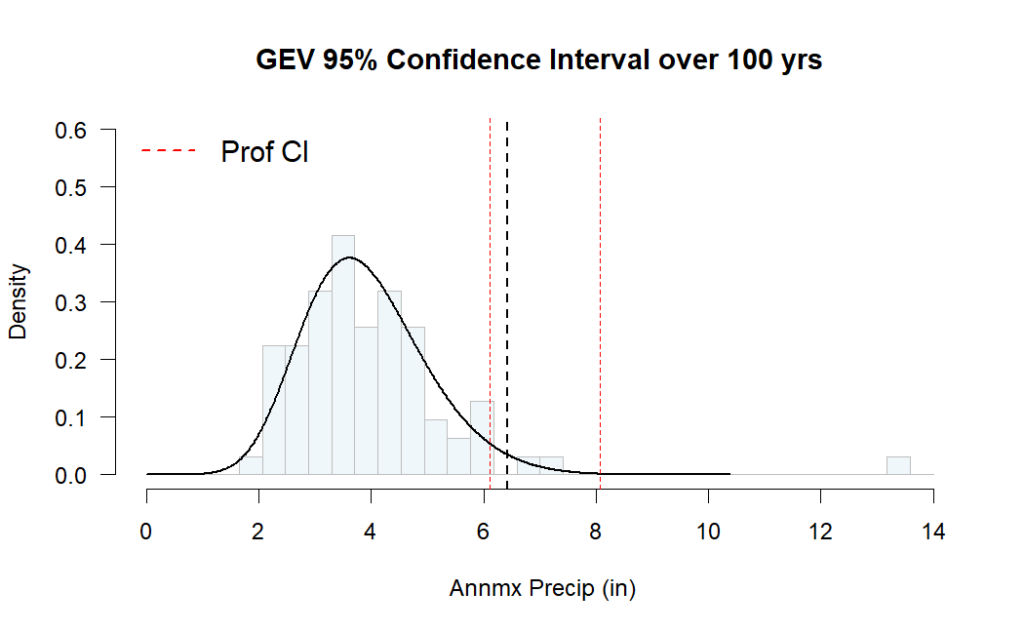
This is the same histogram as the sidebar in the previous plot (note that the bin spacing is not the same) laid out normally, with the predicted 100-year extreme and a 95% confidence band around it. We have a 100-year rain event of 6.4 inches, with a 95% confidence band between 6.1 and 8.2 inches.
Breaking the Model with new Data
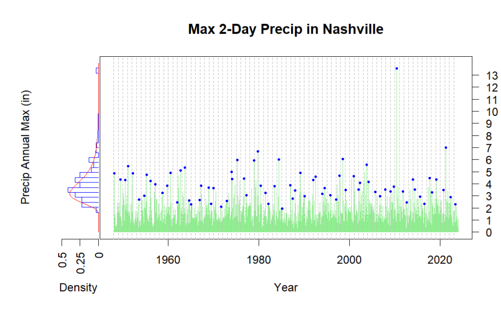
OK, now I’m going to get mean. Nashville was chosen because of a known single super-extreme event. A great real-world example of two-day pairing is the May, 2010, flooding of downtown Nashville. The National Weather Service reports that 7.25” of rain fell on May 2nd, besting the previous record of 6.6 inches. But the two-day total record, adding in 6.32” from May 1st, leapt to 13.57 inches of rain. The previous two-day record was 6.68”, only 0.08” greater than the old one-day record[2].
The previous maximum 2-day rain event was less than seven inches. So now we have a serious outlier to deal with. How will that affect the analysis? The whole set of available rain data is brought in, from 1948 through 2023.

The event from 2010 stands out dramatically. Only one event since has even equaled the old record, about seven inches. The GEV model fit didn’t allow much chance of this happening (it’s beyond the 10,000-year event). But we can at least update the model with the new information and talk about how much smarter we are now.

Our expected 100-year event is now at 6.4 inches of rain, all the way up from 6.4! We might have expected the value to go up, so that’s curious. The good news is we have an even tighter confidence band, ranging from 6.1 to under 8.1 inches (previously 6.1” and 8.2”). How could that super-extreme event not have a greater impact on our analysis?
The new data came with one extreme but a bunch of other new data that looked much like the old. The key assumption of this GEV process is that all the data comes from the same “generator”, the real physical process that makes it happen, imagined as a probability distribution. The weather is not like that! Different storms are made in distinct contexts. The generalized extreme value theorem is not general at all – it applies only to unlikely situations where nothing ever changes and every day is (probabilistically) like the last.
Mathematical rigor cannot keep your house from floating away if the axioms are materially false. But it can fool journalists. In one piece we see a promising headline, “Why the May 2010 flood won’t happen again in our lifetime”. The report goes on to completely fail at both skepticism and probability[3]. The headline is not backed up and is in fact countered by the canned explanation of “1000-year floods.”
Back to Basics
What about that “crude, simple” analysis method we tried at the start?
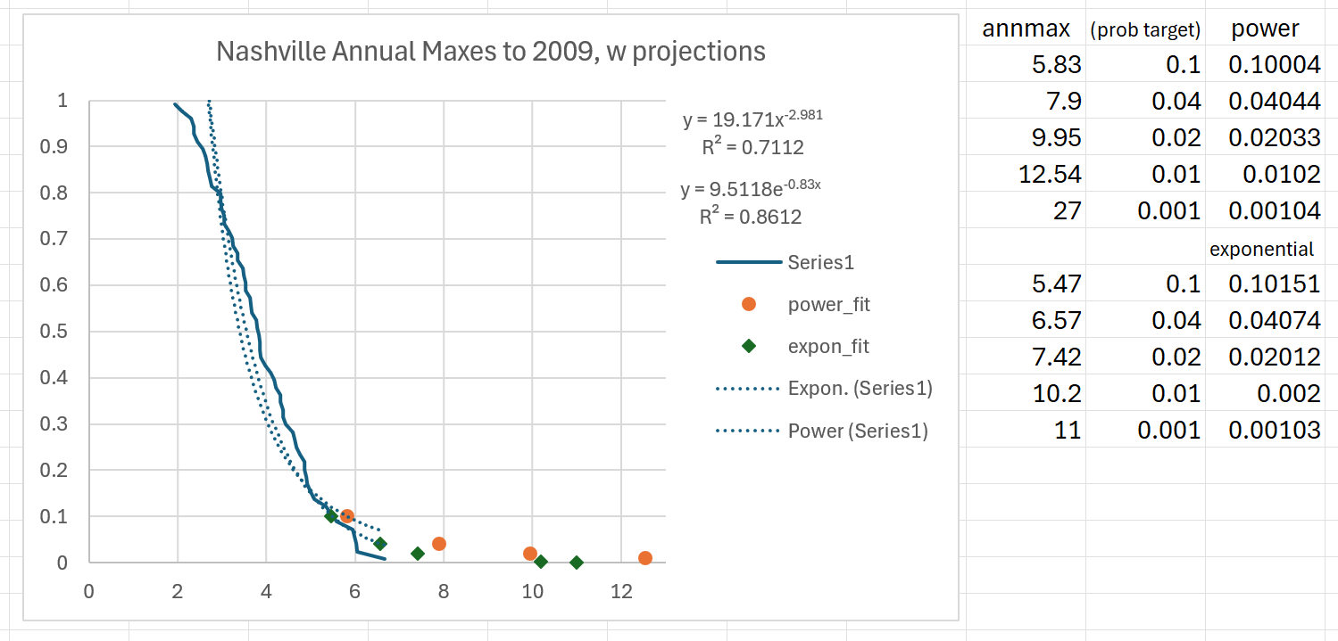
Using just the data through 2009, the sort, plot, and fit routine, all done on a spreadsheet, gives some usable conservative curves.

As usual, the power-law rule fits better and gives more conservative estimates. We have a 100-year event of 12.54 inches (compared to the real 13.57”), and a 1000-year event of a dangerous 27 inches of rain. Numbers like that might have prompted people to build and provide dams and drainage in a very different way.
Which brings us back to the beginning. This all started when the south side of Asheville, North Carolina came to be under ten feet of water. We look at the rain history and how it translates into flooding in the next section.

[1] Code for generating these plots was adapted from materials provided by Professor Whitney Huang, Clemson University.
[2] National Weather Service, (2020), “10th Anniversary of the May 2010 Flood”, https://www.weather.gov/ohx/10thAnniversaryMay2010Flood
[3] Melanie Layden, (May 3, 2024), “Why the May 2010 flood won’t happen again in our lifetime”, https://www.wsmv.com/2024/05/03/why-may-2010-flood-wont-happen-again-our-lifetime/
Next part: https://www.scienceisjunk.com/the-100-year-flood-a-skeptical-inquiry-part-5/
Previous part: https://www.scienceisjunk.com/the-100-year-flood-a-skeptical-inquiry-part-3/